Motivation
If y only takes a finite set of discrete values such as {0,1}, then using Linear Regression to predict a \(\hat y>1/\hat y<0\) does not make sense at all. But fortunately we can fix Linear Regression to produce a value between [0,1].
Details
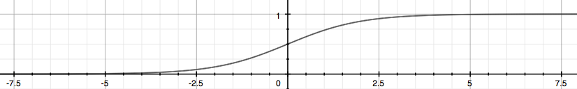
We choose sigmoid/logistic function to map the value: \[h_\theta(x)=g(\theta^Tx),g(z)=\frac{1}{1+e^{-z}}\]
 We can assume that: \[h_\theta(x)=P(y=1|x;\theta)\\
1-h_\theta(x)=P(y=0|x;\theta)\] Or more compactly: \[p(y|x;\theta)=[h_\theta(x)]^y[1-h_\theta(x)]^{1-y}\]
Now we will use maximum likelihood to fit parameters \(\theta\), assume n training examples are
independent, then the likelihood of the parameters is: \[L(\theta)=p(\vec
y|X;\theta)=\prod_{i=1}^{n}p(y^{(i)}|x^{(i)};\theta)=\prod_{i=1}^{n}[h(x^{(i)})]^{y^{(i)}}[1-h(x^{(i)})]^{1-y^{(i)}}\]
To make life easier, we use the log likelihood: \[l(\theta)=log\
L(\theta)=\sum_{i=1}^{n}y^{(i)}log\ h(x^{(i)})+(1-y^{(i)})log\
(1-h(x^{(i)}))\] Let's first take out one example \((x,y)\) to derive the stochastic gradient
ascent rule: \[\frac{\partial}{\partial\theta_j}l(\theta)=[y\frac{1}{g(\theta^Tx)}-(1-y)\frac{1}{1-g(\theta^Tx)}]\frac{\partial}{\partial\theta_j}g(\theta^Tx)
\\=[y\frac{1}{g(\theta^Tx)}-(1-y)\frac{1}{1-g(\theta^Tx)}]g(\theta^Tx)(1-g(\theta^Tx))\frac{\partial}{\partial\theta_j}\theta^Tx
\\=[y(1-g(\theta^Tx))-(1-y)g(\theta^Tx)]x_j=(y-h_\theta(x))x_j\]
Then we can update the parameters: \[\theta_j=\theta_j+\alpha(y^{(i)}-h_{\theta}(x^{(i)}))x_j^{(i)}\]
We can assume that: \[h_\theta(x)=P(y=1|x;\theta)\\
1-h_\theta(x)=P(y=0|x;\theta)\] Or more compactly: \[p(y|x;\theta)=[h_\theta(x)]^y[1-h_\theta(x)]^{1-y}\]
Now we will use maximum likelihood to fit parameters \(\theta\), assume n training examples are
independent, then the likelihood of the parameters is: \[L(\theta)=p(\vec
y|X;\theta)=\prod_{i=1}^{n}p(y^{(i)}|x^{(i)};\theta)=\prod_{i=1}^{n}[h(x^{(i)})]^{y^{(i)}}[1-h(x^{(i)})]^{1-y^{(i)}}\]
To make life easier, we use the log likelihood: \[l(\theta)=log\
L(\theta)=\sum_{i=1}^{n}y^{(i)}log\ h(x^{(i)})+(1-y^{(i)})log\
(1-h(x^{(i)}))\] Let's first take out one example \((x,y)\) to derive the stochastic gradient
ascent rule: \[\frac{\partial}{\partial\theta_j}l(\theta)=[y\frac{1}{g(\theta^Tx)}-(1-y)\frac{1}{1-g(\theta^Tx)}]\frac{\partial}{\partial\theta_j}g(\theta^Tx)
\\=[y\frac{1}{g(\theta^Tx)}-(1-y)\frac{1}{1-g(\theta^Tx)}]g(\theta^Tx)(1-g(\theta^Tx))\frac{\partial}{\partial\theta_j}\theta^Tx
\\=[y(1-g(\theta^Tx))-(1-y)g(\theta^Tx)]x_j=(y-h_\theta(x))x_j\]
Then we can update the parameters: \[\theta_j=\theta_j+\alpha(y^{(i)}-h_{\theta}(x^{(i)}))x_j^{(i)}\]
Here we use maximum likelihood to get the update rule. Generally we would like to minimize the object function. So we can add a negative sign to the maximum likelihood's formula, it is called logistic loss. Thus there exists another way to understand it.
The loss on a single sample can be formulated as follows: \[ cost(h_{\theta}(x),y)=\left\{ \begin{aligned} -log(h_{\theta}(x))\ \ \ if\ y=1\\ -log(1-h_{\theta}(x))\ \ \ if\ y=0 \end{aligned} \right. \] If y=1 and the prediction=1, then loss=0; else if y=1 and the prediction=0, then loss=\(+\infty\) is a huge penalty for the totally wrong prediction. It is the same for y=0.
We can unify the two cases together and the loss for the whole training data is: \[ cost((h_{\theta}(x),y))=-ylog(h_{\theta}(x))-(1-y)log(1-h_{\theta}(x))\\=-\frac{1}{m}\sum_{i=1}^{m}[y^{(i)}log(h_{\theta}(x^{(i)}))+(1-y^{(i)})log(1-h_{\theta}(x^{(i)}))] \] Here the reason why we don't use the MSE loss such as Linear Regression is that the \(J(\theta)\) is non-convex and very hard to optimize for the global optimum.
To make life easier again, we can write the formula as the vectorized version: \[h = g(X\theta),J(\theta) = \frac{1}{m} \cdot \left(-y^{T}\log(h)-(1-y)^{T}\log(1-h)\right)\] Then our goal is to minimize \(J(\theta)\) and get appropriate parameters \(\theta\) and use \(h_\theta(x)=\frac{1}{1+e^{-\theta^Tx}}\) to get our predictions.
Since it is a little complex to get answer analytically, so we still use Gradient Descent to minimize the loss numerically. The update rule is the same as the above one: \[ \theta_j=\theta_j+\alpha\frac{1}{m}\sum_{i=1}^{m}(y^{(i)}-h_{\theta}(x^{(i)}))x_j^{(i)} \] Here you should notice that all \(\theta_j\) should be updated simultaneously when you program. Again the vectorized version: \[\theta=\theta-\frac{\alpha}{m}X^T[g(X\theta)-y]\] It is the same formula as the Linear Regression except that \(h_\theta(x)\) is different.
牛顿法
除了用梯度上升法去最大化\(l(\theta)\),牛顿迭代法也能干这件事。
普通同学都是在求方程的零点\(f(\theta)=0\)时接触到牛顿法,其更新规则为:
\[\theta=\theta-\frac{f(\theta)}{f^{'}(\theta)}\]
这个规则可以理解为:我们一直在用一个线性函数去近似\(f\),因此希望下一次迭代的\(\theta\)就是该线性函数的零点: 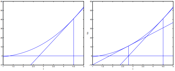 再结合一点高中数学,\(l(\theta)\)极大值点处的一阶导数为0,因此只要令\(l^{'}(\theta)=0\)就能解出对应的\(\theta\): \[\theta=\theta-\frac{l^{'}(\theta)}{l^{''}(\theta)}\]
由于逻辑回归中\(\theta\)是向量而非scalar,因此需要稍稍改变下更新规则:
\[\theta=\theta-H^{-1}\nabla_{\theta}l(\theta)\]
其中,Hessian阵中的元素为\(H_{ij}=\frac{\partial^2l(\theta)}{\partial\theta_i\partial\theta_j}\)。
再结合一点高中数学,\(l(\theta)\)极大值点处的一阶导数为0,因此只要令\(l^{'}(\theta)=0\)就能解出对应的\(\theta\): \[\theta=\theta-\frac{l^{'}(\theta)}{l^{''}(\theta)}\]
由于逻辑回归中\(\theta\)是向量而非scalar,因此需要稍稍改变下更新规则:
\[\theta=\theta-H^{-1}\nabla_{\theta}l(\theta)\]
其中,Hessian阵中的元素为\(H_{ij}=\frac{\partial^2l(\theta)}{\partial\theta_i\partial\theta_j}\)。
牛顿法通常比梯度上升收敛快得多,因为利用了\(l(\theta)\)的二阶信息,但是存储和求解\(H^{-1}\)开销会比较大。